Lecture 8: Hypothesis testing
Economics 326 — Introduction to Econometrics II
Hypothesis testing
Hypothesis testing is one of the fundamental problems in statistics.
A hypothesis is (usually) an assertion about the unknown population parameters such as \beta _{1} in Y_{i}=\beta _{0}+\beta _{1}X_{i}+U_{i}.
Using the data, the econometrician has to determine whether an assertion is true or false.
Example: Phillips curve: \text{Unemployment}_{t}=\beta _{0}+\beta _{1}\text{Inflation}_{t}+U_{t}.
In this example, we are interested in testing if \beta _{1}=0 (no Phillips curve) against \beta _{1}<0 (Phillips curve).
Null and alternative hypotheses
Usually, we have two competing hypotheses, and we want to draw a conclusion, based on the data, as to which of the hypotheses is true.
Null hypothesis, denoted as H_{0}: A hypothesis that is held to be true, unless the data provides sufficient evidence against it.
Alternative hypothesis, denoted as H_{1}: A hypothesis against which the null is tested. It is held to be true if the null is found false.
Usually, the econometrician has to carry the “burden of proof,” and the case that he is interested in is stated as H_{1}.
The econometrician has to prove that his assertion (H_{1}) is true by showing that the data rejects H_{0}.
The two hypotheses must be disjoint: it should be the case that either H_{0} is true or H_{1} but never both simultaneously.
Decision rule
The econometrician has to choose between H_{0} and H_{1}.
The decision rule that leads the econometrician to reject or not to reject H_{0} is based on a test statistic, which is a function of the data \left\{ \left( Y_{i},X_{i}\right) :i=1,\ldots, n\right\} .
Usually, one rejects H_{0} if the test statistic falls into a critical region. A critical region is constructed by taking into account the probability of making a wrong decision.
Errors
There are two types of errors that the econometrician can make:
Truth: H_0 Truth: H_1 Decision: H_0 \checkmark Type II error Decision: H_1 Type I error \checkmark Type I error is the error of rejecting H_{0} when H_{0} is true.
The probability of Type I error is denoted by \alpha and called significance level or size of a test: P\left( \text{Type I error}\right) =P\left( \text{reject }H_{0}|H_{0}\text{ is true}\right) =\alpha .
Type II error is the error of not rejecting H_{0} when H_{1} is true.
Power of a test: 1-P\left( \text{Type II error}\right) =1-P\left( \text{Do not reject }H_{0}|H_{0}\text{ is false}\right) .
Errors
The decision rule depends on a test statistic T.
The real line is split into two regions: acceptance region and rejection region (critical region).
When T is in the acceptance region, we do not reject H_{0} (and risk making a Type II error).
When T is in the rejection (critical) region, we reject H_{0} (and risk making a Type I error).
Unfortunately, the probabilities of Type I and II errors are inversely related. By decreasing the probability of Type I error \alpha , one makes the critical region smaller, which increases the probability of the Type II error. Thus, it is impossible to make both errors arbitrarily small.
By convention, \alpha is chosen to be a small number, for example, \alpha =0.01,0.05, or 0.10. (This is in agreement with the econometrician carrying the burden of proof).
Steps
The following are the steps of the hypothesis testing:
Specify H_{0} and H_{1}.
Choose the significance level \alpha .
Define a decision rule (critical region).
Perform the test using the data: given the data compute the test statistic and see if it falls into the critical region.
The decision depends on the significance level \alpha: larger values of \alpha correspond to bigger critical regions (probability of Type I error is larger).
It is easier to reject the null for larger values of \alpha.
p-value: Given the data, the smallest significance level at which the null can be rejected.
Assumptions
- Recall: under the Normal Classical Linear Regression model and conditionally on \mathbf{X}: \begin{align*} &\hat{\beta}_{1}\sim N\left( \beta _{1},\mathrm{Var}\left(\hat{\beta}_{1} \mid \mathbf{X}\right) \right), \\ &\mathrm{Var}\left(\hat{\beta}_{1} \mid \mathbf{X}\right) =\frac{\sigma ^{2}}{\sum_{i=1}^{n}\left( X_{i}-\bar{X}\right) ^{2}}. \end{align*}
Two-sided tests
For Y_{i}=\beta _{0}+\beta _{1}X_{i}+U_{i}, consider testing H_{0}:\beta _{1}=\beta _{1,0}, against H_{1}:\beta _{1}\neq \beta _{1,0}.
\beta _{1} is the true unknown value of the slope parameter.
\beta _{1,0} is a known number specified by the econometrician. (For example, \beta _{1,0} is zero if you want to test \beta _{1}=0).
Such a test is called two-sided because the alternative hypothesis H_{1} does not specify in which direction \beta _{1} can deviate from the asserted value \beta _{1,0}.
Two-sided test (\sigma^2 known)
Suppose for a moment that \sigma ^{2} is known.
Consider the following test statistic: \begin{align*} &T=\frac{\hat{\beta}_{1}-\beta _{1,0}}{\sqrt{\mathrm{Var}\left(\hat{\beta}_{1} \mid \mathbf{X}\right) }}, \\ &\text{where } \mathrm{Var}\left(\hat{\beta}_{1} \mid \mathbf{X}\right) =\frac{\sigma ^{2}}{\sum_{i=1}^{n}\left( X_{i}-\bar{X}\right) ^{2}}. \end{align*}
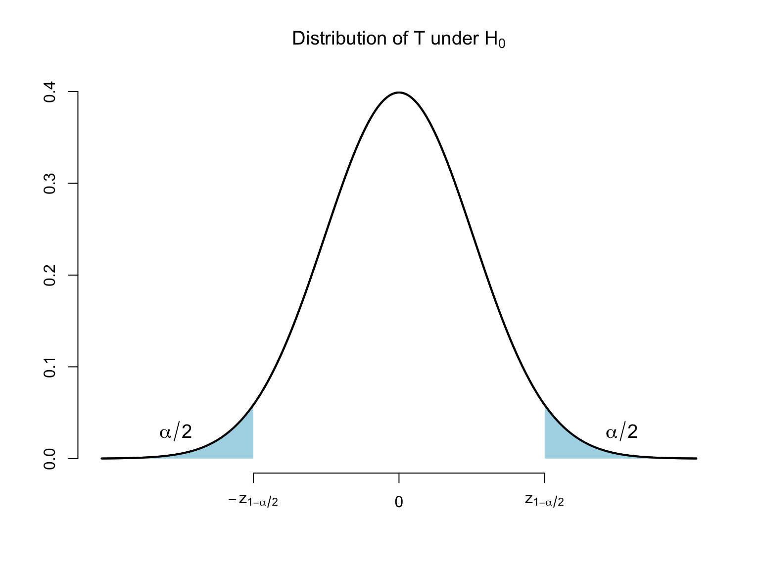
Consider the following decision rule (test): \text{Reject }H_{0}:\beta _{1}=\beta _{1,0}\text{ when }\left\vert T\right\vert >z_{1-\alpha /2}, where z_{1-\alpha /2} is the \left( 1-\alpha /2\right) quantile of the standard normal distribution (critical value).
Test validity and power
We need to establish that:
The test is valid, where the validity of a test means that it has correct size or P\left( \text{Type I error}\right) =\alpha: P\left( \left\vert T\right\vert >z_{1-\alpha /2}|\beta _{1}=\beta _{1,0}\right) =\alpha .
The test has power: when \beta _{1}\neq \beta _{1,0} (H_{0} is false), the test rejects H_{0} with probability that exceeds \alpha: P\left( \left\vert T\right\vert >z_{1-\alpha /2}|\beta _{1}\neq \beta _{1,0}\right) >\alpha .
We want P\left( \left\vert T\right\vert >z_{1-\alpha /2}|\beta _{1}\neq \beta _{1,0}\right) to be as large as possible.
Note that P\left( \left\vert T\right\vert >z_{1-\alpha /2}|\beta _{1}\neq \beta _{1,0}\right) depends on the true value \beta _{1}.
Distribution of T (\sigma^2 known)
Write \begin{align*} T &=\frac{\hat{\beta}_{1}-\beta _{1,0}}{\sqrt{\mathrm{Var}\left(\hat{\beta}_{1} \mid \mathbf{X}\right) }}=\frac{\hat{\beta}_{1}-\beta _{1}+\beta _{1}-\beta _{1,0}}{\sqrt{\mathrm{Var}\left(\hat{\beta}_{1} \mid \mathbf{X}\right) }} \\ &=\frac{\hat{\beta}_{1}-\beta _{1}}{\sqrt{\mathrm{Var}\left(\hat{\beta}_{1} \mid \mathbf{X}\right) }}+\frac{\beta _{1}-\beta _{1,0}}{\sqrt{\mathrm{Var}\left(\hat{\beta}_{1} \mid \mathbf{X}\right) }}. \end{align*}
Under our assumptions and conditionally on \mathbf{X}: \begin{align*} &\hat{\beta}_{1}\sim N\left( \beta _{1},\mathrm{Var}\left(\hat{\beta}_{1} \mid \mathbf{X}\right) \right), \\ &\text{or } \frac{\hat{\beta}_{1}-\beta _{1}}{\sqrt{\mathrm{Var}\left(\hat{\beta}_{1} \mid \mathbf{X}\right) }}\sim N\left( 0,1\right) . \end{align*}
We have that conditionally on \mathbf{X}: T\sim N\left( \frac{\beta _{1}-\beta _{1,0}}{\sqrt{\mathrm{Var}\left(\hat{\beta}_{1} \mid \mathbf{X}\right) }},1\right) .
Size of the test (\sigma^2 known)
Conditionally on \mathbf{X}, we have that T\sim N\left( \frac{\beta _{1}-\beta _{1,0}}{\sqrt{\mathrm{Var}\left(\hat{\beta}_{1} \mid \mathbf{X}\right) }},1\right) .
When H_{0}:\beta _{1}=\beta _{1,0} is true, T\overset{H_{0}}{\sim }N\left( 0,1\right) conditionally on \mathbf{X}.
We reject H_{0} when \left\vert T\right\vert >z_{1-\alpha /2}\Leftrightarrow T>z_{1-\alpha /2}\text{ or }T<-z_{1-\alpha /2}.
Let Z\sim N\left( 0,1\right) . \begin{align*} P\left( \text{Reject }H_{0}|H_{0}\text{ is true}\right) &=P\left( Z>z_{1-\alpha /2}\right) +P\left( Z<-z_{1-\alpha /2}\right) \\ &=\alpha /2+\alpha /2=\alpha \end{align*}
Distribution of T (\sigma^2 known)
Power (\sigma^2 known)
Under H_{1}, \beta _{1}-\beta _{1,0}\neq 0 and, conditionally on \mathbf{X}, the distribution of T is not centered at zero: T\sim N\left( \frac{\beta _{1}-\beta _{1,0}}{\sqrt{\mathrm{Var}\left(\hat{\beta}_{1} \mid \mathbf{X}\right) }},1\right) .
When \beta _{1}-\beta _{1,0}>0:
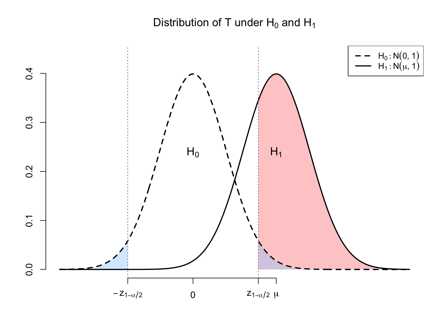
Rejection probability exceeds \alpha under H_{1}: power increases with the distance from H_{0} (\left\vert \beta _{1,0}-\beta _{1}\right\vert) and decreases with \mathrm{Var}\left(\hat{\beta}_{1} \mid \mathbf{X}\right).
The two-sided t-test
We are testing H_{0}:\beta _{1}=\beta _{1,0} against H_{1}:\beta _{1}\neq \beta _{1,0}.
When \sigma ^{2} is unknown, we replace it with s^{2}=\frac{1}{n-2}\sum_{i=1}^{n}\hat{U}_{i}^{2}.
Recall the standard error of \hat{\beta}_{1}: \mathrm{se}\left(\hat{\beta}_{1}\right) = \sqrt{\widehat{\mathrm{Var}}\left(\hat{\beta}_{1}\right)} = \sqrt{\frac{s^{2}}{\sum_{i=1}^{n}\left( X_{i}-\bar{X}\right) ^{2}}}.
The t-statistic: T=\frac{\hat{\beta}_{1}-\beta _{1,0}}{\mathrm{se}\left(\hat{\beta}_{1}\right)}.
We also replace the standard normal critical values z_{1-\alpha /2} with the t_{n-2} critical values t_{n-2,1-\alpha /2}.
However, for large n, t_{n-2,1-\alpha /2}\approx z_{1-\alpha /2}.
The two-sided t-test: \text{Reject }H_{0}\text{ when }\left\vert T\right\vert >t_{n-2,1-\alpha /2}.
The two-sided p-value
The decision to reject or not reject H_{0} depends on the critical value t_{n-2,1-\alpha /2}.
If \alpha _{1}>\alpha _{2} then t_{n-2,1-\alpha _{1}/2}<t_{n-2,1-\alpha _{2}/2}.
Thus, it is easier to reject H_{0} with the significance level \alpha _{1} since it corresponds to a smaller acceptance region.
p-value is the smallest significance level \alpha for which we can reject H_{0}.
The two-sided p-value
In order to find the p-value:
Compute T.
The p-value = 2 \cdot P(t_{n-2} \leq -|T|).
In R:
2 * pt(-abs(T), df = n - 2).
Note that for all \alpha >p-value, \left\vert T\right\vert =t_{n-2,1-\left( p\text{-value}\right) /2}>t_{n-2,1-\alpha /2} and we will reject H_{0}.
For all \alpha \leq p-value, \left\vert T\right\vert =t_{n-2,1-\left( p\text{-value}\right) /2}\leq t_{n-2,1-\alpha /2} and we will not reject H_{0}.
Example of p-value calculation
Suppose a regression with 19 observations produced the following output:
Coefficients:
            Estimate Std. Error t value Pr(>|t|)
(Intercept) 10.18197    0.25094   40.58   <2e-16 ***
x           -0.67253    0.58049   -1.16    0.263
Here, \hat{\beta}_{1}=-0.6725,\beta _{1,0}=0, and the
t valuecolumn gives t=-0.6725/0.5804=-1.16.Thus, \left\vert T\right\vert =1.16 and df=17.
The two-sided p-value:
2 * pt(-abs(-1.16), df = 17)[1] 0.2620816The p-value is large, so we cannot reject H_{0} at conventional significance levels.
Computing in R
We compute critical values and p-values using R.
To compute standard normal quantiles use
qnorm(τ), where \tau is a number between 0 and 1:# z critical value for a two-sided 5% test qnorm(1 - 0.05 / 2)[1] 1.959964For t critical values use
qt(τ, df), where df is the number of degrees of freedom and \tau is the left-tail probability:# t critical value for a two-sided 5% test with 62 df qt(1 - 0.05 / 2, df = 62)[1] 1.998972
Computing in R
To compute two-sided normal p-values use
2 * pnorm(-abs(T)):# Two-sided normal p-value for T = 1.96 2 * pnorm(-abs(1.96))[1] 0.04999579To compute two-sided t-distribution p-values, use
2 * pt(-abs(T), df):# Two-sided t p-value for T = 1.96 with 62 df 2 * pt(-abs(1.96), df = 62)[1] 0.05449415
Example
Data:
rentalfrom thewooldridgeR package. 64 US cities in 1990.rent: average monthly rent ($)avginc: per capita income ($)
Model: Rent_{i}=\beta _{0}+\beta _{1}AvgInc_{i}+U_{i}.
Regression output:
library(wooldridge)
data("rental")
rental90 <- subset(rental, y90 == 1)
reg <- lm(rent ~ avginc, data = rental90)
summary(reg)$coefficients
Estimate Std. Error t value Pr(>|t|) (Intercept) 148.77643972 32.097874358 4.635087 1.885260e-05 avginc 0.01158001 0.001308365 8.850748 1.340614e-12R reports the t-statistics and the p-value for H_{0}:\beta_1 =0.
To test H_{0} whether the coefficient of AvgInc is zero: T=0.01158/0.0013084=8.85.
The p-value is extremely close to zero:
2 * pt(-abs(8.85), df = 62)[1] 1.344588e-12So for all reasonable significance levels \alpha , we reject H_{0} that the coefficient of AvgInc is zero.
AvgInc is a statistically significant regressor.
Example (continued)
Consider now testing H_{0} that the coefficient of AvgInc is 0.009 against the alternative that it is different from 0.009.
T=\left( 0.01158-0.009\right) /0.0013084\approx 1.97.
T_stat <- (0.01158 - 0.009) / 0.0013084
T_stat
[1] 1.971874At 5% significance level, t_{62,0.975}\approx 1.999>T and we do not reject H_{0}.
qt(0.975, df = 62)[1] 1.998972At 10% significance level, t_{62,0.95}\approx 1.67<T and we reject H_{0}.
qt(0.95, df = 62)[1] 1.669804The two-sided p-value:
2 * pt(-abs(T_stat), df = 62)[1] 0.05308963The p-value is \approx 0.053.
For \alpha \leq 0.053 we will not reject H_{0} and for \alpha >0.053 we will reject H_{0}.
Confidence intervals and hypothesis testing
There is a one-to-one correspondence between confidence intervals and hypothesis testing.
We cannot reject H_{0}:\beta _{1}=\beta _{1,0} against a two-sided alternative if \left\vert T\right\vert \leq t_{n-2,1-\alpha /2}, i.e., if and only if: \begin{align*} &-t_{n-2,1-\alpha /2}\leq \frac{\hat{\beta}_{1}-\beta _{1,0}}{\mathrm{se}\left(\hat{\beta}_{1}\right)}\leq t_{n-2,1-\alpha /2} \\ &\Longleftrightarrow \\ &\hat{\beta}_{1}-t_{n-2,1-\alpha /2} \times \mathrm{se}\left(\hat{\beta}_{1}\right) \\ &\qquad \leq \beta _{1,0}\leq \hat{\beta}_{1}+t_{n-2,1-\alpha /2} \times \mathrm{se}\left(\hat{\beta}_{1}\right) \\ &\Longleftrightarrow \\ &\beta _{1,0}\in CI_{1-\alpha }. \end{align*}
Thus, for any \beta _{1,0}\in CI_{1-\alpha }, we cannot reject H_{0}:\beta _{1}=\beta _{1,0} against H_{1}:\beta _{1}\neq \beta _{1,0} at significance level \alpha .
Example
The 95% confidence interval for the coefficient of AvgInc:
confint(reg, "avginc", level = 0.95)2.5 % 97.5 % avginc 0.008964625 0.01419539A significance level 5% test of H_{0}:\beta _{1}=\beta _{1,0} against H_{1}:\beta _{1}\neq \beta _{1,0} will not reject H_{0} if \beta _{1,0} is in the 95% confidence interval.
One-sided tests
Consider testing H_{0}:\beta _{1}\leq \beta _{1,0} against H_{1}:\beta _{1}>\beta _{1,0}.
It is reasonable to reject H_{0} when \hat{\beta}_{1}-\beta _{1,0} is large and positive or when T=\frac{\hat{\beta}_{1}-\beta _{1,0}}{\mathrm{se}\left(\hat{\beta}_{1}\right)}>c_{1-\alpha } where c_{1-\alpha} is a positive constant.
The null hypothesis H_{0} is composite. The probability of rejection under H_{0} depends on \beta _{1}.
We pick the critical value c_{1-\alpha} so that P\left( \frac{\hat{\beta}_{1}-\beta _{1,0}}{\mathrm{se}\left(\hat{\beta}_{1}\right)}>c_{1-\alpha }|\beta _{1}\leq \beta _{1,0}\right) \leq \alpha for all \beta _{1}\leq \beta _{1,0}.
One-sided tests
- For all \beta _{1}\leq \beta _{1,0}, \frac{\beta _{1}-\beta _{1,0}}{\mathrm{se}\left(\hat{\beta}_{1}\right)}\leq 0, and \begin{align*} &P\left( \frac{\hat{\beta}_{1}-\beta _{1,0}}{\mathrm{se}\left(\hat{\beta}_{1}\right)}>c_{1-\alpha }|\beta _{1}\leq \beta _{1,0}\right) \\ &=P\left( \frac{\hat{\beta}_{1}-\beta _{1}}{\mathrm{se}\left(\hat{\beta}_{1}\right)}+\frac{\beta _{1}-\beta _{1,0}}{\mathrm{se}\left(\hat{\beta}_{1}\right)}>c_{1-\alpha }|\beta _{1}\leq \beta _{1,0}\right) \\ &\leq P\left( \frac{\hat{\beta}_{1}-\beta _{1}}{\mathrm{se}\left(\hat{\beta}_{1}\right)}>c_{1-\alpha }|\beta _{1}\leq \beta _{1,0}\right) \\ &=\alpha \text{ if }c_{1-\alpha }=t_{n-2,1-\alpha }. \end{align*}
One-sided tests
For size \alpha test, we reject H_{0}:\beta _{1}\leq \beta _{1,0} against H_{1}:\beta _{1}>\beta _{1,0} when T=\frac{\hat{\beta}_{1}-\beta _{1,0}}{\mathrm{se}\left(\hat{\beta}_{1}\right)}>t_{n-2,1-\alpha }, where t_{n-2,1-\alpha} is the critical value corresponding to the t-distribution with n-2 degrees of freedom.
- Note that we use 1-\alpha and not 1-\alpha /2 for choosing critical values in the case of one-sided testing.
For size \alpha test, we reject H_{0}:\beta _{1}\geq \beta _{1,0} against H_{1}:\beta _{1}<\beta _{1,0} when T=\frac{\hat{\beta}_{1}-\beta _{1,0}}{\mathrm{se}\left(\hat{\beta}_{1}\right)}<-t_{n-2,1-\alpha }.
One-sided tests
One-sided p-values for H_{0}:\beta _{1}\leq \beta _{1,0} against H_{1}:\beta _{1}>\beta _{1,0}:
Compute T.
The p-value = P(t_{n-2} \geq T) = 1 - P(t_{n-2} \leq T).
In R:
1 - pt(T, df = n - 2).